Gaussopt Example

The GaussOpt package can be used to analyze quasioptical systems using Gaussian beam analysis.

This simple example will walk through the basics of setting up a Gaussian beam telescope.

%matplotlib inline

from gaussopt import *

import matplotlib.pyplot as plt
from IPython.display import Image

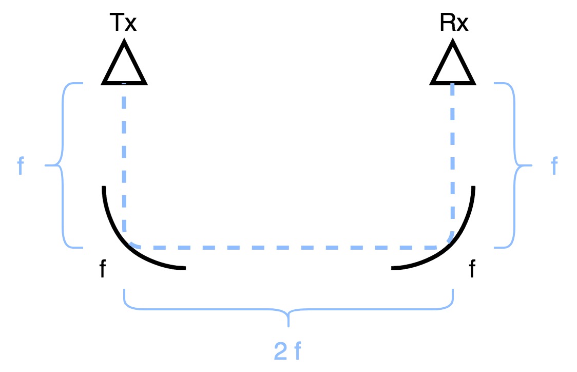
Gaussian beam telescopes use two mirrors to couple energy between two horn antennas. If the mirrors have focal lengths \(f\), then the mirrors should be separated by \(2\,f\) and the distance between each horn’s beam waist and its respective mirror should be \(f\).

Define frequency sweep

Here we will define a frequency sweep from 150 GHz to 300 GHz using the gaussopt.Frequency class.

Note that this class assumes units of GHz unless a different unit is provided.

freq = Frequency(150, 300)

Frequency sweep:
        f = 150.0 to 300.0 GHz, 301 pts

Define horns

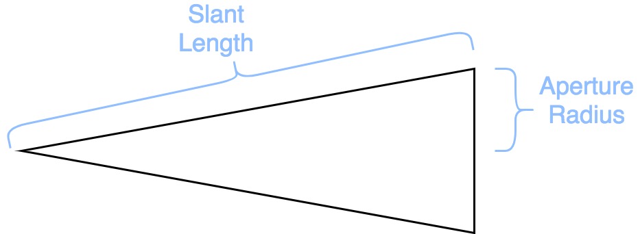
As seen in the figure below, horn antennas are defined by their slant length, aperture radius and horn factor. See "Quasioptical Systems" by Paul Goldsmith for more information. We will use the gaussopt.Horn class to generate the transmitting horn (horn_tx) and then copy this horn to generate the receiving horn (horn_rx).

title

slen = 22.64  # slant length (in mm)
arad = 3.6    # aperture radius (in mm)
hfac = 0.59   # horn factor

horn_tx = Horn(freq, slen, arad, hfac, comment='Trasmitting')
horn_rx = horn_tx.copy(comment='Receiving')

Horn: Trasmitting
        slen = 22.64 mm
        arad =  3.60 mm
        hf   =  0.59

Horn: Receiving
        slen = 22.64 mm
        arad =  3.60 mm
        hf   =  0.59

Define optical components

Now it is time to build the rest of the circuit, i.e., everything between the transmitting and receiving horns. We can define empty space using the gaussopt.Freespace class and mirrors using the gaussopt.Mirror class.

d = Freespace(160)
m1 = Mirror(16, units='cm', radius=8, comment='M1')
m2 = Mirror(16, units='cm', radius=8, comment='M2')

Freespace:
        d = 160.0 mm

Mirror: M1
        f = 16.0 cm

Mirror: M2
        f = 16.0 cm

Note that the distance between a horn and a mirror needs to be reduced because the actual beam waist will be behind the horn aperture.

z_offset = horn_tx.z_offset(units='mm')[freq.idx(230)]
d_red = Freespace(160 - z_offset, comment='reduced')

Freespace: reduced
        d = 155.8 mm

Build Optical System

We can now combine all of the individual optical components to build our optical system. This is normally done by creating a list of optical components (component_list below), starting from the transmitting horn and then listing each component to the receiving horn.

The component list is then passed to the gaussopt.System class, along with the two horns, to calculate the system properties.

component_list = (d_red, m1, d, d, m2, d_red)

system = System(horn_rx, component_list, horn_tx)

System:
[[-1.          0.00848684]
 [ 0.         -1.        ]]

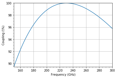
Plot Coupling

The coupling between the two horns can be plotted using the plot_coupling method. There should be perfect coupling at the center frequency.

system.plot_coupling()
system.print_best_coupling()

Best coupling: 100.0 % at 230.0 GHz

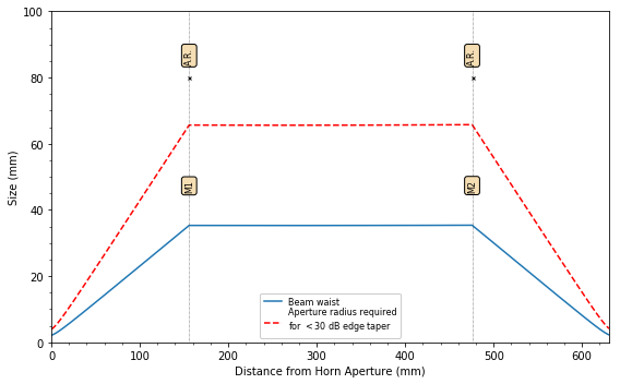
Plot Beam Propagation

The beam waist can be plotted through the entire chain using the plot_system command. This method will also plot the aperture of each component to ensure that there isn’t too much edge taper anywhere in the system.

fig, ax = plt.subplots(figsize=(8,5))
system.plot_system(ax=ax)