4. Example #2: Simulating an SIS mixer
This example will simulate a simple SIS mixer.
The input will consists of 3 signals:
a strong local-osciallator (LO) signal at 230 GHz,
a weak RF signal at 232 GHz, and
an IF output at 2 GHz.
An arbitrary embedding circuit is included (therefore, harmonic balance is required).
The response function is generated from an experimental DC I-V curve.
This simulation will calculate:
the pumped I-V curve, and
the mixer’s gain.
[1]:
%matplotlib inline

import qmix
import numpy as np
import scipy.constants as sc
import matplotlib.pyplot as plt

from qmix.mathfn.misc import slope
from qmix.qtcurrent import qtcurrent
from qmix.circuit import EmbeddingCircuit
from qmix.harmonic_balance import harmonic_balance

# https://github.com/garrettj403/SciencePlots
plt.style.use(['science', 'notebook'])
4.1. Define the junction properties
These are common parameters that describe the electrical properties of SIS junctions. QMix only uses normalized values, so these values will be used to de-normalize whatever voltages, currents and frequencies that QMix calculates.
[2]:
vgap = 2.7e-3              # gap voltage in [V]
rn   = 13.5                # normal resistance in [ohms]
igap = vgap / rn           # gap current in [A]
fgap = sc.e * vgap / sc.h  # gap frequency in [Hz]
4.2. Define the embedding circuit
We will load the
EmbeddingCircuitclass with all of the information about the embedding circuit. This includes the Thevenin voltage, the Thevenin impedance, and the frequency of each signal that is applied to the junction.Note:
All of the circuit properties are normalized:
voltages are normalized to the gap voltage (
vgap),resistances to the normal resistance (
rn),currents to the gap current (
igap = vgap / rn), andfrequencies to the gap frequency (
fgap).
This example includes the embedding circuit. Each tone/harmonic requires:
the Thevenin voltage (normalized to
vgap)the Thevenin impedance (normalized to
rn)the frequency (normalized to
fgap).
The normalized frequency is the same thing as the normalized photon voltage.
[4]:
# simulation parameters
num_f = 3  # number of tones
num_p = 1  # number of harmonics
num_b = (10, 5, 10)  # Bessel function summation limits

# LO signal
f_lo         = 230e9 / fgap      # frequency (normalized value)
alpha_lo     = 1.2               # junction drive level (normalized value)
impedance_lo = 0.3 - 0.3*1j      # embedding impedance (normalized value)

# RF signal
f_rf         = 232e9 / fgap      # frequency (normalized value)
alpha_rf     = 0.012             # junction drive level (normalized value)
impedance_rf = 0.3 - 0.3*1j      # embedding impedance (normalized value)

# IF signal
f_if         = 2e9 / fgap        # frequency (normalized value)
impedance_if = 1.                # embedding impedance (normalized value)

# build embedding circuit
cct = EmbeddingCircuit(num_f, num_p, fgap=fgap, vgap=vgap, rn=rn)
cct.comment[1][1] = 'LO'
cct.comment[2][1] = 'USB'
cct.comment[3][1] = 'IF'

# photon voltages (same as normalized frequency)
cct.freq[1] = f_lo
cct.freq[2] = f_rf
cct.freq[3] = f_if

# Thevenin voltages
cct.vt[1, 1] = cct.freq[1] * alpha_lo
cct.vt[2, 1] = cct.freq[2] * alpha_rf
cct.vt[3, 1] = 0.

# Thevenin impedances
cct.zt[1, 1] = impedance_lo
cct.zt[2, 1] = impedance_rf
cct.zt[3, 1] = impedance_if

cct.print_info()
Embedding circuit (Tones:3, Harmonics:1)
   f=1, p=1                 230.0 GHz x 1           LO
        Thev. voltage:          0.4228 * Vgap
                                1.2000 * Vph
        Thev. impedance:        0.30-0.30j * Rn
        Avail. power:           4.02E-08 W
                                -43.956 dBm
   f=2, p=1                 232.0 GHz x 1           USB
        Thev. voltage:          0.0043 * Vgap
                                0.0120 * Vph
        Thev. impedance:        0.30-0.30j * Rn
        Avail. power:           4.09E-12 W
                                -83.881 dBm
   f=3, p=1                 2.0 GHz x 1             IF
        Thev. voltage:          0.0000 * Vgap
                                0.0000 * Vph
        Thev. impedance:        1.00+0.00j * Rn
        Avail. power:           0.00E+00 W
                                -inf dBm
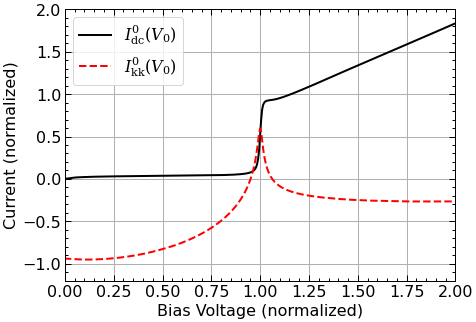
4.3. Generate the response function
Here, the response function is generated from an experimental DC I-V curve.
[5]:
# Load DC I-V data
dciv = qmix.exp.RawData0('example-data/dciv.csv')

# Grab response function
resp = dciv.resp
DC I-V data:
        Vgap:             2.72  mV
        fgap:           658.72  GHz

        Rn:              13.41  ohms
        Rsg:            368.05  ohms
        Q:               27.44

        Jc:              13.54  kA/cm^2
        Ileak:            8.71  uA

        Offset:           0.10  mV
                          9.67  uA

        Vint:             0.45  mV
[6]:
# Plot
fig, ax = plt.subplots(figsize=(7,5))
resp.plot(ax=ax);
4.4. Perform harmonic balance
Calculate the voltage drop across the junction for each tone/harmonic using harmonic balance.
[7]:
vj = harmonic_balance(cct, resp, num_b)
Running harmonic balance:
 - 3 tone(s) and 1 harmonic(s)
 - 7 calls to the quasiparticle tunneling current (qtc) function per iteration
 - max. iterations: 10
Estimated time:
 - time per qtc call:     0.09 s /   0.00 min /  0.00 hrs
 - time per iteration:    0.61 s /   0.01 min /  0.00 hrs
 - max sim time:          6.07 s /   0.10 min /  0.00 hrs
Error after 0 iteration(s):
        f:1, p:1,   med. rel. error:     0.248,   max. rel. error:     1.013,     0.0 % complete
        f:2, p:1,   med. rel. error:     0.213,   max. rel. error:     0.768,     0.0 % complete
        f:3, p:1,   med. rel. error: 99999.999,   max. rel. error: 99999.999,     0.0 % complete
Calculating inverse Jacobian |--------------------| 100.0% Complete
Applying correction
Error after 1 iteration(s):
        f:1, p:1,   med. rel. error:     0.003,   max. rel. error:     0.134,    29.4 % complete
        f:2, p:1,   med. rel. error:     0.011,   max. rel. error:     0.235,    14.9 % complete
        f:3, p:1,   med. rel. error:     0.117,   max. rel. error:    18.770,     0.0 % complete
Calculating inverse Jacobian |--------------------| 100.0% Complete
Applying correction
Error after 2 iteration(s):
        f:1, p:1,   med. rel. error:     0.000,   max. rel. error:     0.003,    99.5 % complete
        f:2, p:1,   med. rel. error:     0.000,   max. rel. error:     0.005,    98.0 % complete
        f:3, p:1,   med. rel. error:     0.000,   max. rel. error:     0.304,    88.1 % complete
Calculating inverse Jacobian |--------------------| 100.0% Complete
Applying correction
Error after 3 iteration(s):
        f:1, p:1,   med. rel. error:     0.000,   max. rel. error:     0.000,   100.0 % complete
        f:2, p:1,   med. rel. error:     0.000,   max. rel. error:     0.000,   100.0 % complete
        f:3, p:1,   med. rel. error:     0.000,   max. rel. error:     0.000,   100.0 % complete
Done: Minimum error target was achieved.
 - sim time:               2.08 s /   0.03 min /  0.00 hrs
 - 3 iterations required
 - time per iteration:     0.69 s /   0.01 min /  0.00 hrs
4.5. Calculate tunnelling currents
idcis the DC tunneling currentilois the AC tunneling current at the LO frequencyiifis the AC tunneling current at the IF frequency
[9]:
freq_list = [0., f_lo, f_if]
idc, ilo, iif = qtcurrent(vj, cct, resp, freq_list, num_b=num_b)
Calculating tunneling current...
 - 3 tone(s)
 - 1 harmonic(s)
Done.
Time: 0.2079 s
4.5.1. Calculate mixer gain
[10]:
# Available power from upper sideband (USB)
pusb = cct.available_power(f=2)

# Power delivered to load
rload = cct.zt[3,1].real * rn
pload = 0.5 * np.abs(iif * igap)**2 * rload

# Gain
gain = pload / pusb
4.6. Plot Results
[11]:
# Conversion: normalized -> de-normalized
vmv = vgap / sc.milli
iua = igap / sc.micro
[12]:
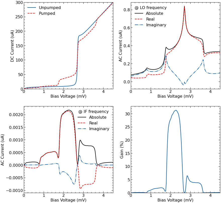
fig, ((ax1, ax2), (ax3, ax4)) = plt.subplots(2, 2, figsize=(14,14))

# Plot I-V curves
ax1.plot(resp.voltage*vmv, resp.current*iua, label='Unpumped')
ax1.plot(cct.vb*vmv, idc.real*iua, 'r--', label='Pumped')
ax1.set(xlim=(0,4.5), xlabel='Bias Voltage (mV)')
ax1.set(ylim=(0,300), ylabel='DC Current (uA)')
ax1.legend(frameon=False)

# Plot AC currents at LO frequency
ax2.plot(cct.vb*vmv, np.abs(ilo), 'k', label='Absolute')
ax2.plot(cct.vb*vmv, ilo.real, 'r--', label='Real')
ax2.plot(cct.vb*vmv, ilo.imag, ls='-.', label='Imaginary')
ax2.set(xlim=(0,4.5), xlabel='Bias Voltage (mV)')
ax2.set(ylabel='AC Current (uA)')
ax2.legend(frameon=False, loc=2, title="@ LO frequency")

# Plot AC currents at IF frequency
ax3.plot(cct.vb*vmv, np.abs(iif), 'k', label='Absolute')
ax3.plot(cct.vb*vmv, iif.real, 'r--', label='Real')
ax3.plot(cct.vb*vmv, iif.imag, ls='-.', label='Imaginary')
ax3.set(xlim=(0,4.5), xlabel='Bias Voltage (mV)')
ax3.set(ylabel='AC Current (uA)')
ax3.legend(frameon=False, loc=1, title="@ IF frequency")

# Plot gain of SIS junction
ax4.plot(cct.vb*vmv, gain*100)
ax4.set(xlim=(0,4.5), xlabel='Bias Voltage (mV)')
ax4.set(ylabel='Gain (%)')
ax4.set_ylim(bottom=0)

fig.savefig('multi-tone-results.png', dpi=500, bbox_inches='tight');