3. Example #1: Creating a simple 1 tone simulation

• This notebook contains a very simple SIS simulation:

  • The input consists of only one tone and one harmonic

  • The embedding circuit is ignored (i.e., no harmonic balance is required)

  • The DC current-voltage relationship is generated through a polynomial model

• The simulation then calculates:

  • The DC tunneling current (i.e., the pumped I-V curve)

  • The AC tunneling current

%matplotlib inline

import qmix
import numpy as np
import matplotlib.pyplot as plt

# https://github.com/garrettj403/SciencePlots
plt.style.use(['science', 'notebook'])

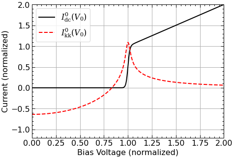
3.1. Generate the response function

• Here we will generate the response function using the polynomial model from Kennedy (1999).

• The RespFnPolynomial class will automatically generate the Kramers-Kronig transform of the DC I-V curve, and then setup the interpolation.

resp = qmix.respfn.RespFnPolynomial(p_order=50)

# Plot
fig, ax = plt.subplots(figsize=(7,5))
resp.plot(ax=ax);

Generating response function:
 - Interpolating:
        - DC I-V curve:
                - npts for DC I-V: 273
                - avg. error: 3.7010E-10
                - max. error: 0.0000 at v=-1.10
        - KK curve:
                - npts for KK I-V: 330
                - avg. error: 6.1923E-07
                - max. error: 0.0001 at v=1.11

3.2. Define embedding circuit

The EmbeddingCircuit class contains all of the information about the embedding circuit. This includes the Thevenin voltages, the Thevening impedances, and the frequencies of the applied signals. In this notebook, the Thevenin impedance is ignored. This means that the AC voltage across the junction is equal to the Thevenin voltage of the embedding circuit (no harmonic balance required).

• Note:

  • All of the circuit properties are normalized:

    • voltages are normalized to the gap voltage (vgap),

    • resistances to the normal resistance (rn),

    • currents to the gap current (igap = vgap / rn), and

    • frequencies to the gap frequency (fgap).

# Create an instance of the embedding circuit class
cct = qmix.circuit.EmbeddingCircuit()

# Set the normalized photon voltage
# (equivalent to the normalized frequency)
cct.freq[1] = 0.33

# Set the Thevenin voltage
cct.vt[1, 1] = 0.33

# Calculate AC voltage across junction
vj = qmix.harmonic_balance.harmonic_balance(cct, resp)

Running harmonic balance:
Done.

3.3. Calculate desired tunnelling currents

qmix.qtcurrent.qtcurrent will calculate the quasiparticle tunnelling current based on the voltage across the junction vj, the simulation parameters contained within cct, and the response function resp.

• Note:

  • The frequency that it solves for is the last argument passed to the function below. For example,

    • 0 corresponds to the DC quasiparticle tunnelling current

    • cct.freq[1] corresponds to the AC quasiparticle tunnelling current of the first tone and first harmonic

# DC tunneling current
idc = qmix.qtcurrent.qtcurrent(vj, cct, resp, 0)

# AC tunneling current
iac = qmix.qtcurrent.qtcurrent(vj, cct, resp, cct.freq[1])

Calculating tunneling current...
 - 1 tone(s)
 - 1 harmonic(s)
Done.
Time: 0.0041 s

Calculating tunneling current...
 - 1 tone(s)
 - 1 harmonic(s)
Done.
Time: 0.0030 s

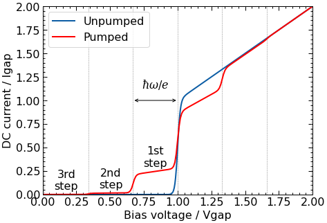
3.4. Plot the pumped I-V curve

fig, ax = plt.subplots(figsize=(7,5))

# vertical lines for photon steps
for i in range(-10, 10):
    ax.axvline(1 - i * cct.freq[1], c='gray', ls='--', lw=0.5)

# plot I-V data
ax.plot(resp.voltage, resp.current, label='Unpumped')
ax.plot(cct.vb, idc, 'r', label='Pumped')

# label the steps
for i, lbl in zip(range(3), ['1st', '2nd', '3rd']):
    vtmp = 1 - (i + 0.5) * cct.freq[1]
    itmp = np.interp(vtmp, cct.vb, idc)
    ax.annotate("{}\nstep".format(lbl),
                xy=(vtmp, itmp+0.15),
                xytext=(vtmp, itmp+0.15),
                va='center', ha='center',
                fontsize=16)
# hw/e label
ax.text(1-cct.freq[1]/2, 1.1, r'$\hbar\omega/e$', fontsize=16, ha='center', va='bottom')
ax.annotate("", xy=(1-cct.freq[1], 1), xytext=(1, 1),
    arrowprops=dict(arrowstyle="<->", color='k'))

# other labels
ax.set(xlabel='Bias voltage / Vgap', xlim=[0,2])
ax.set(ylabel='DC current / Igap', ylim=[0,2])
ax.legend(frameon=True);

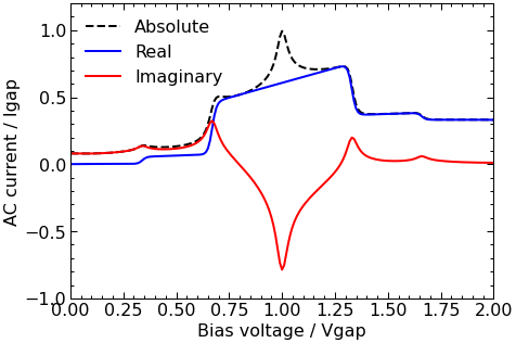
3.5. Plot the AC tunneling currents

fig, ax = plt.subplots(figsize=(7,5))

ax.plot(cct.vb, np.abs(iac), 'k--', label=r'Absolute')
ax.plot(cct.vb, np.real(iac), 'b', label=r"Real")
ax.plot(cct.vb, np.imag(iac), 'r', label=r"Imaginary")
ax.set(xlabel='Bias voltage / Vgap', xlim=[0,2])
ax.set(ylabel='AC current / Igap', ylim=[-1,1.2])
ax.legend(frameon=False);